Yuan and Kopp (2021)

Title:

Emulating Ocean Dynamic Sea Level by Two-Layer Pattern Scaling

Key Points:

• An emulator for DSL changes is developed based on a two-layer energy balance model and a two-layer pattern scaling technique

• The two-layer emulator can better capture the evolution of DSL in corresponding coupled GCMs than scaling of global mean surface temperature

• The two-layer emulator allows estimation of the probability of future DSL changes in various emission scenarios over multiple centuries

Corresponding author:

10. Yuan

Citation:

Yuan, J., & Kopp, R. E. (2021). Emulating ocean dynamic sea level by two-layer pattern scaling. Journal of Advances in Modeling Earth Systems, 13, e2020MS002323, https://doi.org/10.1029/2020MS002323

URL:

https://agupubs.onlinelibrary.wiley.com/doi/10.1029/2020MS002323

Abstract

Ocean dynamic sea level (DSL) change is a key driver of relative sea level (RSL) change. Projections of DSL change are generally obtained from simulations using atmosphere-ocean general circulation models (GCMs). Here, we develop a two-layer climate emulator to interpolate between emission scenarios simulated with GCMs and extend projections beyond the time horizon of available simulations. This emulator captures the evolution of DSL changes in corresponding GCMs, especially over middle and low latitudes. Compared with an emulator using univariate pattern scaling, the two-layer emulator more accurately reflects GCM behavior and captures non-linearities and non-stationarity in the relationship between DSL and global-mean warming, with a reduction in global-averaged error during 2271-2290 of 36%, 24%, and 34% in RCP2.6, RCP4.5, and RCP8.5, respectively. Using the emulator, we develop a probabilistic ensemble of DSL projections through 2300 for four scenarios: Representative Concentration Pathway (RCP) 2.6, RCP 4.5, RCP 8.5, and Shared Socioeconomic Pathway (SSP) 3-7.0. The magnitude and uncertainty of projected DSL changes decrease from the high-to the low-emission scenarios, indicating a reduced DSL rise hazard in low- and moderate-emission scenarios (RCP2.6 and RCP4.5) compared to the high-emission scenarios (SSP3-7.0 and RCP8.5).

Plain Language Summary

As climate warms, sea-level rise poses a major threat to coastal communities and ecosystems. A key driver of local sea level change is ocean dynamic sea level change, which is associated with changes in ocean density and circulation. The primary tools used to project changes in dynamic sea level are atmosphere-ocean general circulation models, which are computationally expensive. Here we develop an emulator for dynamic sea level changes that is, built upon a two-layer energy balance model. Considering both the rapid response of well-mixed surface layer and the delayed response of the deep ocean to forcing, the emulator facilitates the estimation of probability distributions of future dynamic sea level change under different emission scenarios and the extension of projections beyond the time horizon of available simulations from some atmosphere-ocean general circulation models. This emulator captures the evolution of dynamic sea level changes in the atmosphere-ocean general circulation models to which it is tuned, including the non-linear and non-stationary relationship between the dynamic sea level and global warming. The emulator thus facilitates the estimation of future local sea-level changes.

Introduction

Sea-level rise impacts coastal communities and ecosystems through permanent inundation, increasingly common tidal flooding, and increasingly frequent and severe storm-driven flooding. Global-mean sea level (GMSL) is rising at an accelerating rate, and under most scenarios is projected to continue accelerating over the 21st century (Oppenheimer et al., 2019). Regional relative sea level (RSL) change differs from global-mean sea-level change due to a variety of processes operating on diverse timescales, including the gravitational, rotational, and deformational effects associated with mass redistribution and ocean dynamic effects associated with changes in surface winds, ocean currents, and heat and freshwater fluxes (Gregory et al., 2016, 2019; Kopp et al., 2015; Perrette et al., 2013; Stammer et al., 2013).

Atmosphere-ocean general circulation models (GCMs) are the primary tool used to project ocean dynamic sea level (DSL) change, but the computational demands of these models limit the utility of GCM ensembles for estimating the likelihood of different levels of future sea-level change. Ensembles such as the Coupled Model Intercomparison Project Phase 5 (CMIP5, Landerer et al., 2014; Taylor et al., 2012) are composed of models contributed based on voluntary effort, not the product of systematic experimental design; as such, they are an “ensemble of opportunity” rather than a probabilistic ensemble (Tebaldi & Knutti, 2007). The CMIP future projection experiments are driven by a small number of forcing scenarios - Representative Concentration Pathways (RCPs) in the case of CMIP5 - and model simulations are of different lengths; some simulations run the RCPs to the year 2100, while others extend these to 2300.

The computationally intensive nature of GCMs makes it challenging to produce large perturbed-physics ensembles that represent uncertainties in key feedback parameters, as well as to simulate forcing conditions intermediate between the RCPs. Simple climate models (SCMs) provide an alternative tool for estimating the uncertainties of future projections at the global scale, as they can capture the overall physics of climate evolution and can be run very fast even on a personal computer (Held et al., 2010; Meinshausen et al., 2011; Millar et al., 2017; Perrette et al., 2013). However, SCMs represent the climate at a highly aggregated (e.g., global or hemispheric) scale, and thus cannot produce spatial patterns of climate change at each time step.

Pattern scaling approaches are often used to translate the global mean surface air temperature (GSAT) change into regional-scale changes for impact analysis (Mitchell, 2003; Rasmussen et al., 2016; Santer, 1990; Tebaldi & Arblaster, 2014; Tebaldi et al.,2011). Generally speaking, pattern scaling uses a simple statistical model (often, linear regression) to relate local climatic changes to a variable such as GSAT change, assum.ing the patterns of local response to external forcing remain constant under increased forcing (Tebaldi & Arblaster, 2014).

Some previous studies use the pattern scaling approach to estimate the uncertainty in DSL projections (Bilbao et al., 2015; M. D. Palmer et al., 2020; Perrette et al., 2013). For example, Perrette et al. (2013) regressed DSL change on GSAT. At New York City, they found that r² values across models vary between 0.02 and 0.85, and also that the linear relationship between DSL and GSAT becomes weaker after the 21st century. Bilbao et al. (2015) examined the relationship between DSL and several variables, including GSAT, global-mean sea-surface temperature, ocean volume mean temperature, and global-mean thermosteric sea-level rise (GMTSLR). They found that GSAT performed best in predicting 21st-century DSL change in a high emissions scenario (RCP 8.5), while ocean-volume mean temperature and GMTSLR performed better in lower emissions scenarios (RCP 2.6 and 4.5). They speculated that this difference reflects a more important role for surface warming relative to deep warming in a more strongly forced scenario. They found that, across models and scenarios, area-weighted average root mean square error in pattern-scaled 2081–2100 DSL change ranged from ~1 to 3 cm.

Building upon Bilbao et al. (2015)’s speculation about the relative importance of shallow and deep warming under different scenarios, we developed a bivariate pattern scaling, which uses a multiple linear regression with two predictors: GSAT and global-mean deep ocean temperature change. The two temperature changes can be generated by a two-layer energy-balance model (2LM) (Held et al., 2010; Winton et al., 2010), which has proved to be a useful tool for understanding the responses of climate system to climate forcing (Geoffroy et al, 2013a, 2013b). Shallow and deep temperatures from a 2LM have previously been employed in an emulator to extend 21st century CMIP5 projections of GMTSLR to 2300 (M. D. Palmer et al., 2018), and M. D. Palmer et al. (2020) used GSAT from the two-layer model and univariate pattern scaling (based on GSAT) to emulate CMIP5 projections of DSL change.

In this study, we develop an emulator for DSL changes using both GSAT and deep-ocean temperature change projected by a 2LM. Here we drive the 2LM with radiative forcings from the Finite Amplitude Impulse Response model (FaIR), a SCM which includes a reduced-complexity carbon cycle and calculates atmospheric CO₂ concentrations, radiative forcing and temperature changes based on emissions (Millar et al., 2017; Smith et al., 2017, 2018). FaIR was designed to more accurately reflect the temporal evolution of GSAT in response to a pulse emission, and it has been used in previous studies to produce observation-constrained future projections (Millar et al., 2017; Smith et al., 2017, 2018). In this study, we develop an emulator for GMTSLR and DSL change using surface and deep-ocean temperature changes generated by the FaIR-2LM (Section 2.2). As the univariate pattern scaling fails to capture the delayed response of the deep ocean to warming, we employ FaIR-2LM and two-layer pattern scaling to project future DSL changes, taking into account uncertainty in climate sensitivity, and demonstrate their ability to interpolate between climate scenarios run by GCMs. Compared to M. D. Palmer et al. (2018, 2020), which also use a 2LM to emulate GMTSLR or DSL projections, our approach differs in: (1) employing radiative forcings calculated based on emissions; (2) applying a format of 2LM considering efficacy factor of deep ocean heat uptake; (3) using both surface and deep-ocean temperature for pattern scaling (more details are described in supporting information).

Section 2 describes data and methodology, including the details of FaIR-2LM, the calibration of the FaIR.2LM based on selected CMIP5 GCMs, the two-layer pattern scaling methodology, and the application of this system to emulate DSL projections. Section 3 evaluates the performance of the two-layer pattern scaling. Section 4 shows the resulting ensemble of DSL projections. Finally, Section 5 discusses and summarizes the results.

Data and Methods

Data

We use the zos variable from five CMIP5 general circulation models (GCMs) in RCP 2.6, 4.5, and 8.5 sce.narios: MPI-ESM-LR, bcc-csm1-1, HadGEM2-ES, GISS-E2-R, IPSL-CM5A-LR. These five GCMs are used because they were used to calibrate the parameters of the 2LM by Geoffroy et al. (2013) and provide multi-century data (to 2300) for zos in all three scenarios. DSL is taken as zos with its global mean removed, consistent with the definition of Gregory et al. (2019). The drift is removed from DSL by subtracting a linear function of time fitted to the pre-industrial control simulation from each scenario experiments, at each grid point. In addition, we remove the climatology in a baseline period (1986-2005) from DSL. The global mean surface air temperature (GSAT) and GMTSLR from the five models in the three scenarios are also used to evaluate the performance of FaIR-2LM.

FaIR-Two Layer Model (FaIR-2LM) and Calibration

This study develops a hybrid SCM model by replacing the temperature module in FaIR 1.3 (Smith et al., 2018) with a 2LM. In FaIR 1.3, GSAT changes are the sum of two components, representing fast and slow responses to effective radiative forcing (ERF) (Equation 22 in Smith et al., 2018). The fast and slow components of temperature changes in FaIR 1.3 mathematically depend on multiple coefficients (e.g., thermal response timescales) that are obtained from the ensemble mean of multiple CMIP5 models (Geoffroy, et al., 2013b). Since these components do not have an unambiguous physical meaning, it is challenging to link them to sea-level change. Therefore, we replace the temperature module in FaIR 1.3 by the 2LM to construct FaIR.2LM. In each step of FaIR-2LM, the 2LM is driven by radiative forcing from FaIR 1.3, and produces the GSAT anomaly, which feeds back to the FaIR carbon cycle (Figure S1).

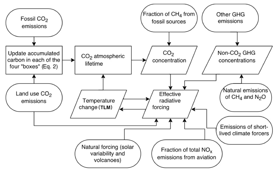
Figure S1: Schematic diagram of the FaIR-2LM (modified from Figure 1 of Smith et al. 2018).

We employ a 2LM that includes an efficacy term for deep ocean heat uptake (Geoffroy, et al., 2013a; Held et al., 2010; Winton et al., 2010):

C frac{dT}{dt} = mathcal{F} - lambda T - epsilon gamma (T - T_0) (1)

C_0 frac{dT_0}{dt} = gamma (T - T_0) (2)

where mathcal{F} denotes the adjusted radiative forcing, C and C_0 are the heat capacity of the well-mixed upper layer and the deep ocean layer, respectively, and T and T_0 represent the global mean temperature anomalies of the upper and lower layer, respectively. Following Equation 22 in Geoffroy, et al. (2013b) and using C = 8.2 W yr m^{-2} K^{-1} and C_0 = 109 W yr m^{-2} K^{-1} based on an average across multiple CMIP5 GCMs (Geoffroy, et al., 2013a), we estimate the average depths of the upper layer and lower layer are 86 m and 1141 m, respectively. T is equivalent to GSAT perturbation (Held et al., 2010). lambda is the parameter for climate feedback, gamme is the coefficient of deep ocean heat uptake, and epsilon is the efficacy factor of deep ocean heat uptake, which represents the uneven spatial distribution of heat exchanges between the two layers.

To calibrate FaIR-2LM, we adjust parameter settings (listed in Table 1) based on previous studies (Forster et al., 2013; Geoffroy, Saint-Martin, et al., 2013a; Zelinka et al., 2014). The radiative forcing in FaIR-2LM is driven by the default emission trajectory for each scenario in FaIR 1.3, but scaled by two parameters determined for each GCM: (1) the radiative forcing of CO_2 doubling (F_{2 times CO_2}) reported by Forster et al. (2013), and (2) the present-day aerosol forcing (a*f_{pd}) estimated in previous studies (Forster et al., 2013; Zelinka et al., 2014), or -0.9 W m^{-2} - the median of range estimated by the Fifth Assessment Report of Intergovernmental Panel on Climate Change (IPCC AR5) (Stocker et al., 2013) - for models not reported in previous studies. The five parameters in Equations 1 and 2 (i.e., lambda, gamma, epsilon, C, C_0) are the same as those in Geoffroy et al. (2013) for the corresponding GCMs.

Table 1: FaIR-2LM Parameters adjusted to match the GSAT in CMIP5 GCMs. \(\lambda\) (W m^-2 K^-1), \(\gamma\) (W m^-2 K^-1), \(\epsilon\), C (W yr m^-2 K^-1), and \(C_0\) (W yr m^-2 K^-1) are reported by Geoffroy et al. (2013). The units for \(F_{2 \times CO_2}\) and \(af_{pd}\) are W m^-2.

CMIP5 GCMs	\(\lambda\)	\(\gamma\)	\(\epsilon\)	C	\(C_0\)	\(F_{2 \times CO_2}\)	\(af_{pd}\)
bcc-csm1-1	1.28	0.59	1.27	8.4	56	3.23	-0.9
GISS-E2-R	2.03	1.06	1.44	6.1	134	3.78	-0.9
HadGEM2-ES	0.61	0.49	1.54	7.5	98	2.93	-1.23
IPSL-CM5A-LR	0.79	0.57	1.14	8.1	100	3.1	-0.68
MPI-ESM-LR	1.21	0.62	1.42	8.5	78	4.09	-0.9

GSAT produced by the calibrated FaIR-2LM is compared with that from the corresponding GCMs in the three scenarios (Fig. S2). For the five GCMs, the GSAT simulated by FaIR-2LM is close to the GSAT from the corresponding GCM, with the root mean square error (RMSE) determined over the entire simulation period in a range of 0.15-0.23 K for RCP2.6, 0.14-0.32 K for RCP4.5, and 0.20-0.43 K for RCP8.5.

GMTSLR is driven by the thermal expansion of sea water volume due to the increase in ocean heat uptake. To calibrate GMTSLR in FaIR-2LM to match a specific GCM, we first correct the drift in the GCM’s GMTSLR field by removing the linear trend in the pre-industrial control simulation, assuming the drift is not sensitive to the external forcing (Hobbs et al., 2016).

Then, we emulate GMTSLR based on the T and T_0 from FaIR-2LM following the approach described in Kuhlbrodt and Gregory (2012):

{GMTSLR} = sigma times (C Delta T + C_0 Delta T_0) (3)

where sigma is the expansion efficiency of heat in units of 10^{-24} m J^{-1}. The sigma value is calibrated by optimizing GMTSLR emulated from FaIR-2LM to match the GMTSLR simulated from the corresponding GCM.

Two-Layer Pattern Scaling

Univariate pattern scaling is based on a linear relation between regional changes in a climate variable (DSL for this study) and global mean responses of climate change, such as GSAT (T):

DSL(t,x,y) = alpha(x,y) T(t) + b(x,y) + epsilon(t,x,y) (4)

where x and y denote longitudes and latitudes, t represents the time, b is an intercept term, and epsilon is the residual term. Here, alpha captures the scaling relationship between DSL and GSAT (Figure 1). The five GCMs agree that the linear response of DSL to surface warming is positive over the Arctic and sub-polar Atlantic, and negative over the southeastern Pacific and the southern areas of Southern Ocean.

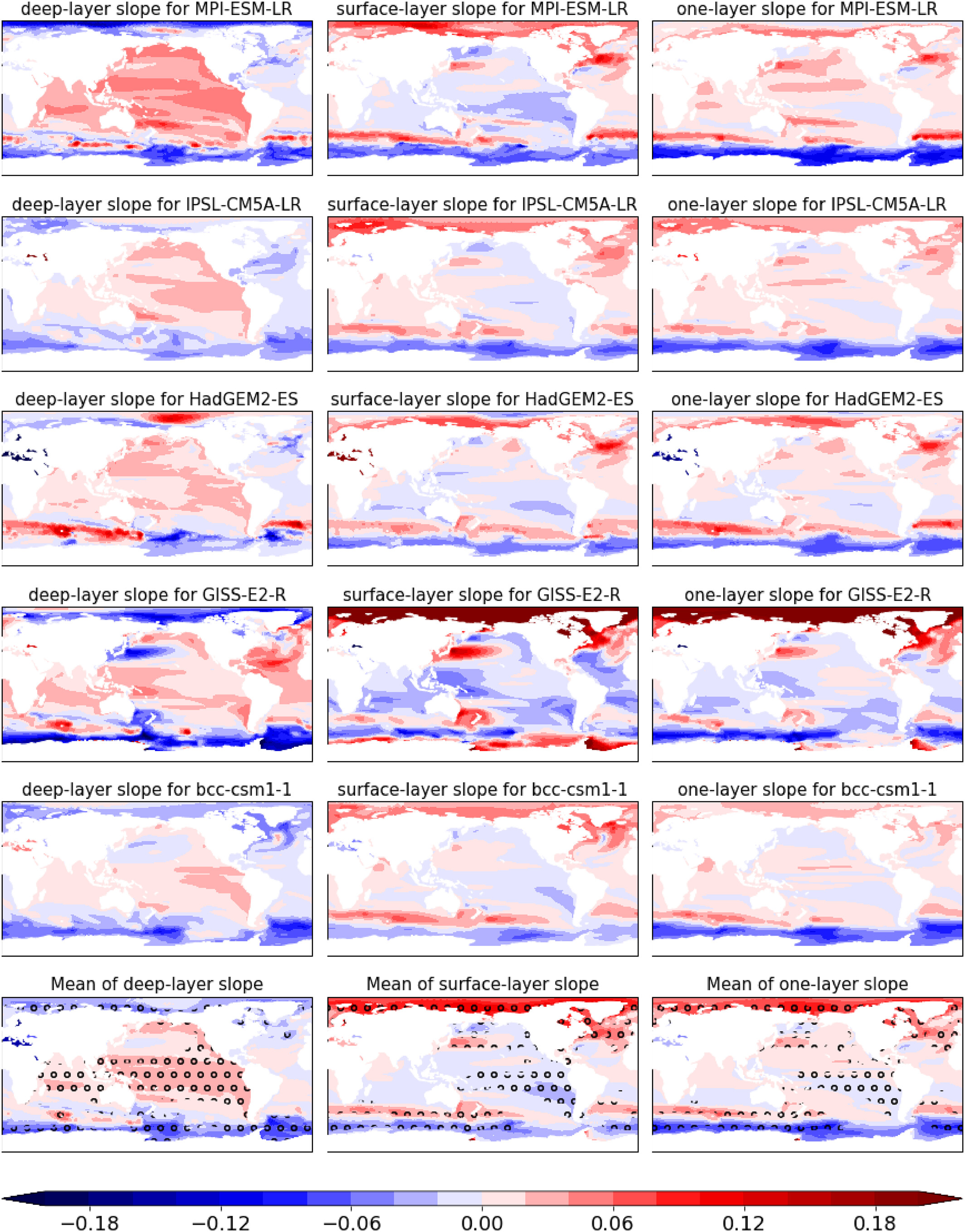
Figure 1: Changes in DSL in response to changes in deep ocean temperature (first column) and global-mean surface air temperature (second column) in bivariate pattern scaling. The third column is the response of DSL changes to global-mean surface air temperature in univariate pattern scaling. The first five rows display the maps of slopes obtained from a GCM over the period of 1981-2300. The sixth row shows the multi-model mean of slopes. The areas where the slopes from the five models agree in sign are hatched. White areas are lands. Units are m K^{-1}.

In the bivariate pattern scaling approach, we regress the DSL anomaly on both T (GSAT anomaly) and T_0 (deep-ocean temperature anomaly) from FaIR-2LM:

DSL(t_i,x,y) = alpha(x,y) T(t_i) + beta(x,y) T_0(t_i) + b(x,y) + epsilon(t,x,y) (5)

where t_i denotes years in three scenarios, i = 1, 2, 3. For each GCM, we estimate the fields of alpha, beta, b, and epsilon by regressing projections from all three emissions scenarios (RCPs 2.6, 4.5, and 8.5) on T and T_0 on a grid cell-by-grid cell basis. alpha represents changes in zos in response to changes in surface temperature in the period 1981–2300, while beta represents the response of changes in zos to changes in deep-ocean temperature at the same period (Figure 1). Consistent with the univariate scaling pattern, the five GCMs agree that the upper-layer response, represented by alpha, is positively correlated with warming over the most areas of Arctic and northern edge of the Southern Ocean, and negatively correlated with warming over the southeastern Pacific and the southern areas of Southern Ocean. The deep-layer response represented by beta is positively correlated with warming over the Indian and tropical and southern Pacific Oceans, and negatively correlated with warming over most areas of the Southern Ocean and Arctic. These reflect opposite behaviors between rapid and sustained changes in DSL over the Arctic, the Indian and tropical and southern Pacific Oceans, and a consistent DSL fall in both rapid and sustained changes over the Southern Ocean.

There is little agreement on either surface- or deep-layer slopes across the five GCMs over most parts of the Atlantic basin (Figure 1). This may reflect limited skill in simulating strong western boundary currents (e.g., the Atlantic Meridional Overturning Circulation (AMOC)) in the GCMs, which have a relatively coarse (~1˚) spatial resolution in ocean component (Small et al., 2014) and so poorly capture non-linear mesoscale processes in the ocean current (Hallberg, 2013). Near the eastern coast of North America, DSL is closely related to AMOC (Goddard et al., 2015), which is expected to weaken in a warming climate (Caesar et al., 2018). Low skill in capturing AMOC behavior can affect the DSL projections in the Atlantic basin as well as its coasts (van Westen et al., 2020). As the coefficients of pattern scaling depend on the simulations by the GCMs, they also do not explicitly resolve the non-linear mesoscale process of the ocean current. Therefore, we should interpret the DSL changes predicted by the two-layer emulator with cautions over the regions where non-linear mesoscale effects of ocean current are strong.

Projecting DSL Using FaIR-2LM and Patterns

We use two steps to generate a probabilistic ensemble of DSL projections. First, we generate an ensemble of surface and deep-ocean temperature pairs using FaIR-2LM. The planetary energy balance at the top of the atmosphere (Zelinka et al., 2020) is:

\[N = \mathcal{F} + \lambda T (6)\]

where N is the radiative imbalance at the top of the atmosphere. The equilibrium climate sensitivity (ECS) is given by T when N = 0, and mathcal{F} = F_{2 times CO_2}. Therefore, lambda is related to F_{2 times CO_2} and ECS by

lambda = - F_{2 times CO_2} / ECS (7)

The uncertainty of F_{2 times CO_2} is small relative to the spread of lambda, while ECS largely determine the uncertainty of lambda. Therefore, we adopt the best estimation in the Intergovernmental Panel on Climate Change Fifth Assessment Report (AR5) for F_{2 times CO_2} = 3.71 W m^{-2} (Collins et al., 2013). We produce initial distributions of ECS, gamma, and gamma_{epsilon} based on the literature constraints (Figure S4) outlined below:

ECS: Based on multiple lines of evidence, the uncertainties of ECS estimated by AR5 are likely in the range 1.5˚C-4.5˚C with high confidence, extremely unlikely less than 1˚C and very unlikely greater than 6˚C (Collins et al., 2013). In the AR5 terminology, likely denotes a probability of at least 66%, very unlikely a probability of less than 10%, and extremely unlikely a probability of less than 5% (Mastrandrea et al., 2010). Therefore, we construct a log-normal distribution for ECS with parameters optimized to match a 5th percentile of 1˚C, a 17th percentile of 1.5˚C, an 83rd percentile of 4.5˚C, and a 90th percentile of 6˚C.

gamma: We treat gamma as normally distribution, with mean 0.67 W m^{-2} K^{-1} and standard deviation 0.15 W m^{-2} K^{-1} derived from the 16 GCMs in the CMIP5 archive (Geoffroy et al., 2013).

gamma_{epsilon}: As the efficacy factor of heat uptake is related to deep-ocean heat uptake (Held et al., 2010), we use gamma_{epsilon} instead of epsilon to maintain the covariance between gamma and epsilon. We calculate the mean of 0.86 W m^{-2} K^{-1} and standard deviation 0.29 W m^{-2} K^{-1} of gamma_{epsilon} based on the products of gamma and epsilon from 16 GCMs in CMIP5 archive (Geoffroy, et al., 2013a). The distribution of gamma_{epsilon} is constructed as a normal distribution with the multi-model mean and the multi-model standard deviation.

TCR: Under a zero-layer approximation which considers the 1%/yr increase in CO_2 until doubling scenario occurring on a timescale long enough that the upper ocean is in approximate equilibrium and short enough that the deep-ocean temperature has not yet responded substantially, Transient Climate Response (TCR) can be obtained by (Jimenez-de-la-Cuesta & Mauritsen, 2019):

{TCR} = - frac{F_{2 times CO_2}}{lambda - gamma_{epsilon}} (8)

Uncertainty in the TCR can be constrained adequately by varying only lambda and gamma_{epsilon} under the zero-layer approximation. Therefore, although there are significant uncertainties of C and C_0 among GCMs, we use fixed values because the uncertainties of these parameters are not necessary to represent uncertainty in the TCR. In this study, we set C = 8.2 W m^{-2} K^{-1} and C_0 = 109 W m^{-2} K^{-1} based on the multi-model mean of GCMs from Coupled Model Intercomparison Project Phase 5 (CMIP5) archive (Geoffroy, et al., 2013a).

We then generate a 100,000-member ensemble of ECS, gamma and gamma_{epsilon} based on these distributions via Monte Carlo sampling. As gamma_{epsilon}} should be larger than 0, we discard parameter sets in which gamma_{epsilon}} < 0 or gamma_{epsilon}} > 2 times 0.86 to keep the mean of gamma_{epsilon}} in parameter sets to be 0.86 W m^{-2} K^{-1}. Therefore, 99734 parameter sets are kept. An ensemble of lambda is then computed by the best estimation of F_{2 times CO_2} and the ensemble of ECS based on Equation 6 (Figure S4). The median (central 66% range) of lambda is −1.39 (−2.4 to −0.8) W m^{-2} K^{-1}. As the likely range of ECS estimated by AR5 is equivalent to the central 90% range of ECS estimated by CMIP5 GCMs, the uncertainty range of lambda estimated by FaIR-2LM is larger than that estimated by ensemble of GCMs (Geoffroy et al., 2013). The spread of TCR is estimated as a diagnostic by substituting the ensemble of lambda, gamma_{epsilon}, and best estimation of F_{2 times CO_2} into Equation 8. The uncertainty of TCR is in a central 66% range of 1.1–2.3˚C, with a 95th percentile of 2.9˚C. This is consistent with but slightly narrower than the TCR estimated by AR5, which is likely between 1˚C and 2.5˚C, and is extremely unlikely greater than 3˚C.

We apply Latin hypercube sampling (LHS, Stein, 1987) to the parameter sets of lambda, gamma, gamma_{epsilon} by sampling 1,000 sets from the 99,734 parameter sets. For each parameter, LHS divides the probability density function of the 99,734 samples into 1,000 portions that have equal area. A sample is taken from each portion randomly so that the 1,000 sample sets cover the multidimensional distribution of the three parameters. Finally, we applied 1,000 parameter sets together with the fixed parameters (F_{2 times CO_2}, C, C0) to the FAIR-2LM and generate a 1,000-member probabilistic ensemble of temperature pair time-series.

We compare the spread in GSAT projected by FaIR-2LM with the likely ranges estimated by AR5 for four different periods (Collins et al., 2013) (Table 3 and Figure S5). The mean of the probabilistic ensemble is slightly lower than the mean estimate of GSAT from AR5 in all four periods of RCP2.6 and RCP4.5, and in the 21st century for RCP8.5. Compared with AR5 likely ranges, the central 66% probability range of GSAT from FaIR-2LM is generally consistent: narrower in all four periods of RCP2.6, narrower in the first two periods but wider in the last two periods in RCP4.5, and wider in the first two periods but narrower in the last two periods in RCP8.5.

We project GMTSLR based on Equation 3 using the probabilistic ensemble of surface and deep-ocean temperature projections from FaIR-2LM. The C, C_0 and expansion efficiency of heat sigma (0.113 times 10^{-24 m}) used here are adopted from the multi-model ensemble mean of CMIP5 archive (Geoffroy, et al., 2013a; Kuhlbrodt & Gregory, 2012).

A projection of DSL is constructed as follows: 1) a pair of alpha and beta is randomly picked with replacement from the pool of two-layer patterns produced in Section 2.3; 2) a temperature pair from the 1000 members is combined with the pair of alpha and beta in an equation:

{DSL}(t, x, y) = alpha(x, y) T(t) + beta(x, y) T_0(t) + b(x, y) (9)

Evaluation of Two-Layer Pattern Scaling

To evaluate the prediction skill of the two-layer pattern scaling, we compare the DSL changes simulated from a GCM with the DSL changes emulated by the two-layer pattern scaling (widehat{{DSL}}) based on FAIR-2LM using the key parameters (i.e. parameters in Table 1) in the same GCM. Two metrics are used: (1) absolute values of the residual differences between widehat{{DSL}} changes and DSL changes during a period at each grid point, and (2) global average of the absolute values obtained from the metric 1 (Table S1). These two metrics are applied to both bivariate pattern scaling and univariate pattern scaling, to examine the improvement of bivariate approach comparing with the univariate approach.

In 2271-2290, for instance, the global-averaged climatology of | DSL - widehat{{DSL}} | (score obtained by the second metric) from the two-layer pattern scaling is less than that from the univariate pattern scaling (bottom row Figure 2), with a reduction of 36%, 24%, and 34% in RCP2.6, RCP4.5, and RCP8.5, respectively. The spatial pattern of R = DSL - widehat{{DSL}} is derived from both approaches are various across GCMs (Figures S6-S10). The 5-model ensemble averaged climatology of | R | in both approaches is higher over high latitudes (e.g., Arctic, subpolar Northern Atlantic, Southern Ocean) than over middle to low latitudes, but is generally lower in two-layer pattern scaling than in univariate pattern scaling (first two rows Figure 2). As the pattern-scaling method cannot resolve DSL change due to unforced variability, the relatively large | R | over the high latitudes may be due to the relatively high unforced variability over these regions (Bilbao et al., 2015).

We further compare the time evolution of widehat{{DSL}} predicted by the two-layer pattern scaling approaches with the evolution of DSL in corresponding GCMs through the period 1981-2290. As case studies, we pick two grid cells: one in the western Pacific near the Philippines (14.5˚N, 127˚E), and the other over the North Atlantic near the coast of New York City [NYC] (40˚N, 73˚W) (solid black dots in Figure 2). The grid point near the Philippines is selected because it is in the tropical Pacific, where DSL rise associated with the deep ocean temperature rise is strongest, while the grid point near the NYC is selected represent a coastal area that some projections find experiences significant DSL changes in response to changes in AMOC.

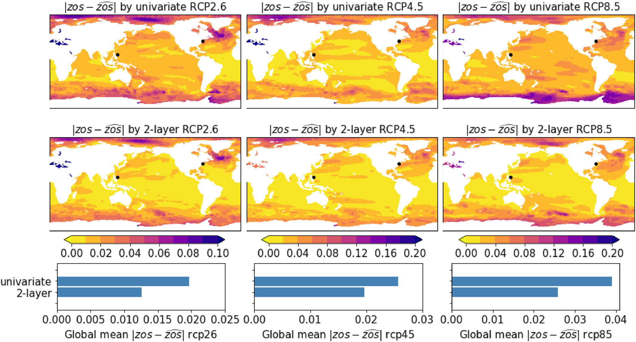
Figure 2: Differences between DSL simulated by GCMs (zos) and DSL (widehat{{zos}}) predicted by univariate pattern scaling (univariate, first row) and two-layer pattern scaling (two-layer, second row) over the period 2271-2290 for the ensemble mean of 5 GCMs in three scenarios: RCP2.6, RCP4.5, RCP8.5 (Units: m). The third row shows the global mean of the | {zos} - (widehat{{zos}} | in 1TS and 2TS, respectively. Black dots on maps denote the two grid cells used for the plot in Figure 3.

At the western Pacific grid cell, in RCP 2.6, the relationship between DSL and GSAT anomaly displays a hook-like shape, indicating continued rise in DSL as GSAT stabilizes and declines in response to negative emissions (Figure 3a). The delayed adjustment of DSL may be due to the continuous warming of deep layer (T_0) when GSAT is stabilized, because the ocean is not yet equilibrated with the elevated forcing. In response to changes in T_0, the deep ocean density is still changing even without changing circulation in the deep ocean (England, 1995), so DSL continues to change. This hook-like shape is captured by the two-layer pattern scaling approach but not by the univariate pattern scaling. Compare to the DSL simulated by a GCM, the RMSE of the predicted DSL is smaller if using the two-layer pattern scaling approach than using the univariate pattern scaling approach. The average RMSE across the five GCMs is reduced 26% if we use the approach from the two-layer pattern scaling instead of the univariate pattern scaling (Table 3). Across the five GCMs, although the relationship between DSL and GSAT is diverse in RCP4.5 and RCP8.5, DSL projected by the two-layer technique is consistently closer than that predicted by the univariate technique to the DSL simulated by the GCMs. The sole exception is for bcc-csm1-1 in RCP8.5, for which the simulated DSL projection is quite linearly associated with GSAT. The average of RMSEs across the 5 GCMs decrease from the univariate pattern scaling approach to the two-layer pattern scaling approach by 35% in RCP4.5 and by 33% in RCP8.5 (Table 3).

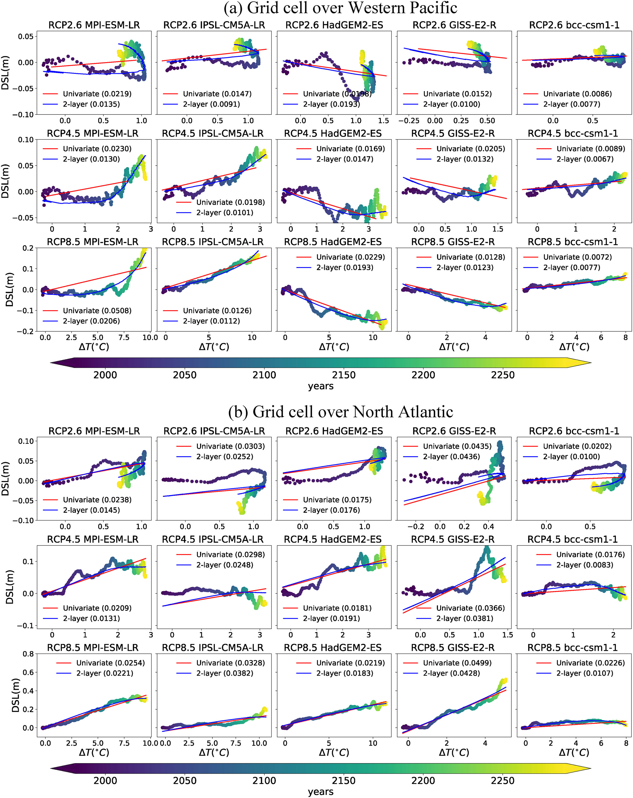
Figure 3: widehat{{zos}} predicted by univariate pattern scaling and two-layer pattern scaling at the grid cell (a) over Western Pacific (14.5˚N, 127˚E) and (b) over the North Atlantic (40˚N, 73˚W) for the five models in the three scenarios. The zos simulated by corresponding GCMs is shown by scatters in which colors indicate years. Root mean square errors between the widehat{{zos}} and zos determined over the entire simulating period for each GCM are shown in parentheses of legend (units: m).

At the North Atlantic grid cell, the relationship between DSL and GSAT also displays non-linear features for all the five models, especially in low- and moderate-emission scenarios (Figure 3b). These non-linear features, which may arise from the delayed response of deep branch of AMOC, cannot be captured by univariate pattern scaling but are captured to a large extent by the two-layer pattern scaling (lines in Figure 3). The value of the two-layer approach is highlighted by the clear non-linearity of the DSL response when viewed as a function of GSAT anomaly. Compare to the univariate approach, the RMSE between the DSL simulated by GCMs and the DSL predicted by the two-layer pattern scaling is smaller, with a reduction of 19%, 16%, and 13% for RCP2.6, RCP4.5, and RCP8.5, respectively. The method of two-layer pattern scaling generally has a better performance in emulating the DSL from the corresponding GCM than the univariate pattern scaling, as the two-layer pattern scaling includes one more predictor than univariate pattern scaling, allowing it to capture the delayed adjustment of DSL. The delayed adjustment of DSL due to the deep-ocean warming is important for the DSL projections, as different areas present different features that may reveal the regional variation in deep-ocean circulation (Held et al., 2010).

Projections of DSL

The procedure described in Section 2.4 allows us to produce a 1000-member probabilistic ensemble of DSL projections not only for the three CMIP5 scenarios: RCP2.6, RCP4.5, and RCP8.5, but also for any other scenarios with an emission pathway between these three scenarios. We demonstrate this capability using SSP3-7.0, a CMIP6 scenario that has forcing intermediate between RCP4.5 and RCP8.5 (O’Neill et al., 2016) and is closer than either to no-policy reference scenarios from most integrated assessment models (Riahi et al., 2017). The emission pathway of SSP3-7.0 used to drive the FaIR-2LM is taken from the Reduced Complexity Model Intercomparison Project (Nicholls et al., 2020).

The five projections using parameters calibrated to the five GCMs respectively are within the 66% range of the 1000-member ensemble for both surface and deep-ocean temperature in the three RCPs (Figure 4). By 2300, the median estimates (66% range) of the surface temperature relative the period of 1986-2005 are 0.5˚C (0.2-1.0˚C) for RCP2.6, 2.2˚C (1.2-3.6˚C) for RCP4.5, 7.4˚C (4.5-11.7˚C for RCP8.5, and 5.3˚C (3.2-8.6˚C) for SSP3-7.0.

Based on the projections of temperature pairs, we also produced projections of GMTSLR for the four scenarios (Figure 4). The spread of GMTSLR ensemble encapsulates the GMTSLR time series from the 5 GCMs (Figure 4). During the period of 2081-2100, the median estimates (66% range) of the GMTSLR relative the period of 1986-2005 are 0.12 (0.07-0.18) m for RCP2.6, 0.16 (0.10-0.24) m for RCP4.5, 0.19 (0.12-0.27) m for SSP3-7.0, and 0.24 (0.15-0.34) m for RCP8.5. This compares to Oppenheimer et al. (2019)’s projected median estimates (66% ranges) of 0.14 (0.10-0.18) m for RCP2.6, 0.19 (0.14-0.23) m for RCP4.5, and 0.27 (0.21-0.33) m for RCP8.5. By 2300, the median estimates (66% range) of GMTSLR relative to the period of 1986-2005 are 0.20 (0.12-0.33) m for RCP2.6, 0.43 (0.25-0.68) m for RCP4.5, 0.85 (0.50-1.33) m for SSP3-7.0, and 1.15 (0.69-1.76) m for RCP8.5. As climate warms, the projections of DSL changes increase along with the increase in GMTSLR. In the five GCMs, although the contributions of DSL changes to the local sterodynamic sea level (DSL+GMTSLR; Gregory et al., 2019) changes are small at some locations (i.e., regions marked by the light and dark gray shadings in Figure S11), in others the ratio of DSL change with respect to the GMTSLR changes are fairly significant. For instance, DSL changes at some regions (e.g., Arctic, North Atlantic, and Southern Ocean) are greater than 50% of the GMTSLR during the period of 2271-2290 (identified by yellow contours in Figure S11).

Figure 4: Ensemble projections of CO_2 concentrations (first row), GSAT (second row), deep-ocean temperature (third row), and GMTSLR (fourth row) changes relative to the baseline period 1986-2005 under the four scenarios. Shadings represents the 66% range, dark blue lines the median of probabilistic ensemble projections. The projection calibrated to the five GCMs in the three RCP scenarios are shown on top of the shadings (orange lines).

Compared with the GSAT and GMTSLR spread in 2300 estimated by M. D. Palmer et al. (2018), the FaIR.2LM projections have a slightly lower median for all the three RCPs. The 66% range of both surface temperature and GMTSLR estimated by FaIR-2LM is comparable to the 90% range of that estimated by M. D. Palmer et al. (2018) because we adopt a distribution of lambda based on the AR5 assessment of equilibrium climate sensitivity (Collins et al., 2012), which is broader than the 90% range estimated by the CMIP5 multi-model ensemble emulated by M. D. Palmer et al. (2018).

Comparing the DSL projections between the period of 2081-2100 and the period of 2271-2290 (Figure 5), the median estimate is lower and the 66% range of uncertainty is narrower at the end of 21st century than that at the end of 23rd century in moderate-to high-emission scenarios (RCP4.5, SSP3-7.0 and RCP8.5). But in RCP2.6, the median estimate and 66% uncertainty range are comparable in magnitude between these two periods. In both periods, the median DSL anomaly projections across the four scenarios share many similar features (Figure 5). Over the Arctic region, a weak increase in DSL is observed over the Chukchi Sea and the Beaufort Sea in RCP2.6. In the higher emission scenarios, the increase in DSL extends to the whole Arctic basin with intensified amplitudes. The changes in DSL over the North Atlantic are dominated by a negative anomaly under RCP2.6, and display positive anomalies over much of the North Atlantic under RCP8.5 and SSP3-7.0. The ensemble spread of the 5th-95th range of DSL projections are relatively large over the Southern Ocean, Arctic and Subpolar Atlantic than other areas. The large uncertainties over these areas, consistent with previous literatures (M. D. Palmer et al., 2020; Perrette et al., 2013; Yin, 2012), may be interpreted by the diverse characteristics simulated by GCMs that do not explicitly resolve non-linear mesoscale processes of the ocean current over these areas (van Westen et al., 2020).

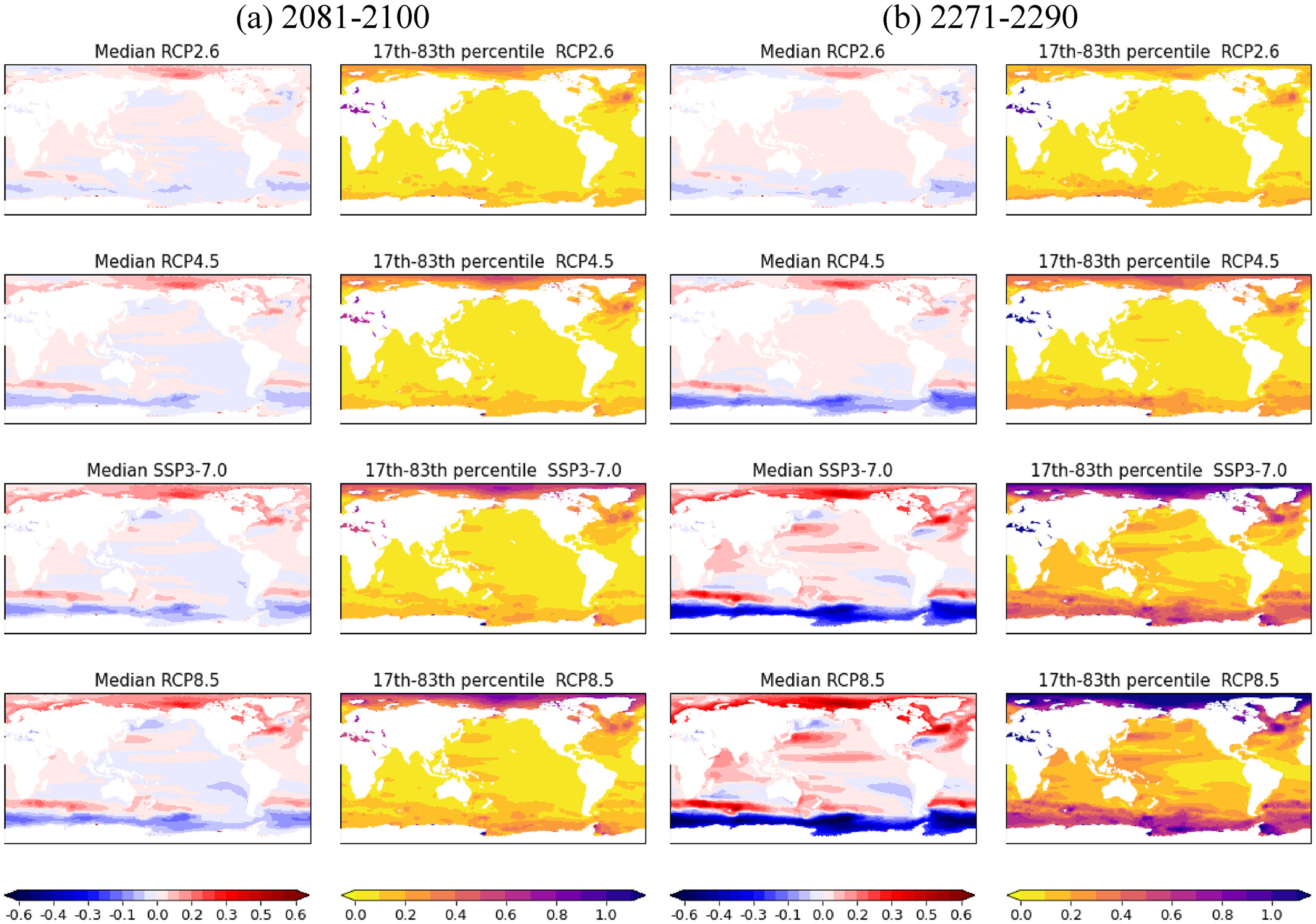
Figure 5: Projection of DSL changes at median estimation (first column) and range of 17th-83rd percentile averaged over the period of 2081-2100 in four scenarios (a) relative to the baseline period 1986-2005. (b) is the same with (a) except for the period of 2271-2290. Units are m.

At the illustrative grid point near Philippines over western Pacific (Figure 6a), the 66% range of the probabilistic ensemble encapsulates DSL projections from 2 of the 5 GCMs in the three RCPs, while the 90% range of the probabilistic ensemble contains DSL projections from all the 5 GCMs in the three RCPs, except for HadGEM2-ES in RCP2.6. At the grid point near NYC, the projected DSL changes estimated by the probabilistic ensemble exhibits a fat tail, with a median projection in RCP 8.5 of 0.13 m and a 95th percentile projection of 0.8 m by the end of 23rd century. By contrast, RCP 2.6 exhibits a much narrower range, with a median of 0 m and a 95th percentile of 0.08 m. The 66% range of the projected DSL uncertainties encapsulates 2 of 5 GCM projections. The 90% range of the probabilistic ensemble only encapsulates the DSL projections from three over five GCMs in RCP2.6 and RCP4.5, but encapsulates the DSL projections from all five GCMs in RCP8.5. The emulator fails to capture multidecadal variability in DSL, a limitation which would be expected because the emulator is constructed based on the pattern scaling approach.

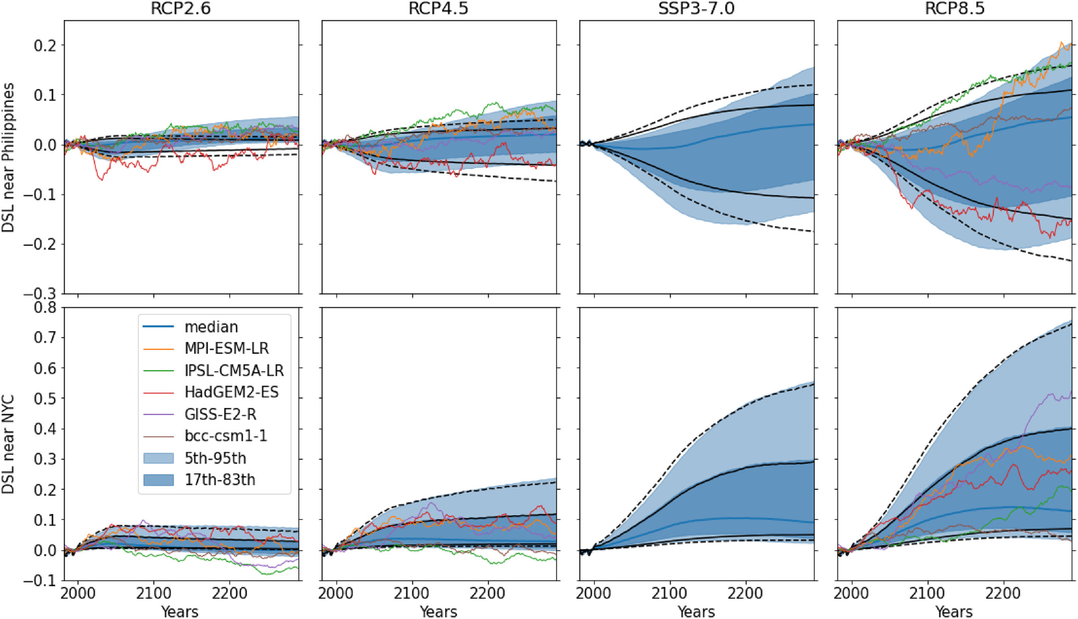
Figure 6: Ensemble projections of DSL changes relative to the baseline period 1986-2005 at the grid cells near Philippines over the western Pacific (upper panel) and near NYC over the North Atlantic (lower panel) for the four scenarios: RCP2.6, RCP4.5, SSP3-7.0, and RCP8.5. Shadings represent the projections produced by the two-layer emulator, with light and dark shadings indicating the 90% and 66% range, respectively, and dark blue lines the median of probabilistic ensemble projections. The black lines represent the projections produced by the univariate emulator, with the dashed and solid lines indicating the 90% and 66% range, respectively. The projection of DSL changes smoothed by 20-years running average in the five GCMs are shown on top of the shadings (colored lines). Units: m.

To compare with the DSL projections derived from two-layer pattern scaling, we also produced the DSL projections based on univariate pattern scaling following the same procedure (Figures S12 and S14). The median and 17th-83rd range of DSL projections derived from univariate pattern scaling are similar in patterns (Figure S12). However, differences of both median and spreads of the DSL projections between univariate and two-layer pattern scaling vary across regions, especially over high latitudes in high-emission scenarios (Figure S13). Specifically, compared to the univariate emulator, the median of DSL projected by the two-layer emulator is lower over the Pacific and Indian Ocean, and higher over Arctic, Atlantic and Southern Ocean in the period of 2081-2100, but the opposite in the period of 2271-2290. In addition, the 17th-83rd range of the DSL projected by the two-layer emulator is wider than that by the univariate emulator over the Arctic. The area-weighted increases in DSL spread over the Arctic are 0.02 m in RCP2.6, 0.03 m in RCP4.5, and 0.04 m in RCP8.5 during 2081-2100, and are 0.006 m in RCP2.6, 0.008 m in RCP4.5, 0.009 m in RCP8.5 during 2271-2290. For the grid cell near Philippines, despite the shift in median, the distributions of DSL projections derived from univariate pattern scaling exhibit a different shape from that derived from two-layer pattern scaling (Figure 6). In 2290, the 90% range of DSL projection from the univariate emulator is close to that from the two-layer emulator, slightly narrower by 0.03 m for RCP2.6, 0.02 m for RCP4.5, and 0.01 m for SSP3-7.0 and RCP8.5. The two-layer pattern scaling leads to not only a shift of the distribution but also a different shape of the distribution of the DSL projections, compared to that derived from univariate pattern scaling. There are more DSL projections simulated by GCMs encapsulated within the 90% range of the probabilistic ensemble of DSL projections derived from two-layer pattern scaling than that by the univariate pattern scaling (Figure 6). For the grid cell near the NYC, the shape of DSL distributions derived from univariate pattern scaling is similar to that derived from two-layer pattern scaling, except the spread of the DSL projections derived from univariate pattern scaling is slightly narrower than that derived from the two-layer pattern scaling, with the 90% range of DSL projection in 2290 narrower by 0.03 m for RCP2.6, 0.01 m for RCP4.5, and 0.03 m for SSP3-7.0 and RCP8.5 (Figure 6). The greatest difference is in RCP 2.6, where the difference in the 90% range is by far the largest compared to the overall range.

Table 2: The Averaged RMSE Between the DSL Simulated by GCMs and the DSL Predicted by Univariate/Two-Layer Pattern Scaling Across Five Models. Note: The averaged RMSEs and the reduction of RMSE from univariate pattern scaling approach to two-layer pattern scaling are calculated for the three RCP scenarios, respectively.

Discussion and Conclusions

We have developed a probabilistic ensemble of DSL projections through 2300 using a novel two-layer emulator. Replacing the climate module in the FaIR simple climate model with a two-layer energy-balance model, we developed FaIR-2LM, which produces projections of global average temperature in the well-mixed upper layer (T) for rapid responses to radiative forcing, and in the deep ocean layer (T_0) for delayed responses. Calibrated by the parameters for each GCMs, the GSAT (Figure S2) and GMTSLR (Figure S3) emulated by FaIR-2LM generally follow that from the corresponding GCM, with RMSE <0.43 K for GSAT and <0.05 m for GMTSLR. A two-layer pattern scaling based on surface and deep-ocean temperature is used to project DSL. During the period 2271-2290, for instance, the DSL predicted by the two-layer pattern scaling are closer to the DSL simulated by the corresponding GCM than that predicted by the univariate pattern scaling (Figure 2). At two selected grid cells (near the coast of Philippines and NYC), the time evolution of DSL projections predicted by the two-layer emulator more accurately reflects GCM behavior and captures non-linearities and non-stationarity in the relationship between DSL and global-mean warming, comparing with that predicted by the univariate technique (Figure 3).

Table 3: Comparison of the Distributions of GSAT Anomaly (Relative to 1986-2005) Projected by FaIR-2LM With the Distributions of Global-Mean Surface Temperature Assessed by AR5 (Collins et al., 2013) in RCP 2.6, RCP4.5, SSP3-7.0 and RCP 8.5 (the 2nd and 3rd Columns, units: ˚C). Note: Means are given without parentheses; likely range (for AR5) and 17th-83rd percentile range (for FaIR-2LM) are given in parentheses. The fourth column is similar with previous columns except for the GMTSLR projected by FAIR-2LM (Units: m).

By perturbating the key parameters, FaIR-2LM allows emulation of projected global-mean surface and deep-ocean temperature pairs and GMTSLR for emissions scenarios (e.g., SSP3-7.0; Figures 4 and 5) beyond those run by the GCMs to which it is calibrated. Compared with the likely ranges assessed by AR5 in the RCP 2.6, 4.5 and 8.5, the FaIR-2LM performs well in emulating the GSAT spread (Table 2 and Figure S5). By 2300, the ensembles of GSAT and GMTSLR estimated by FaIR-2LM have a slightly lower median and a slightly wider 90% range than the estimations by M. D. Palmer et al. (2018), likely because we use the uncertainty of ECS from AR5, which has a larger range than that estimated by CMIP5 multi-model ensemble.

We produce probabilistic ensembles of DSL projections for four different emissions scenarios. Characteristics of median DSL projections during 2271-2290 include increases in DSL along most of the coast around the Pacific and Indian Oceans and a decrease in DSL over the Southern Ocean in all four scenarios, as well as increased DSL over the Arctic and along the North Atlantic Current in moderate to high emissions scenarios (Figure 5). The 66% range (17th-83rd percentile) of uncertainties are small over the middle and low latitudes, and are relatively large over the Southern Ocean, Arctic and North Atlantic, where the simulations of GCMs are diverse due to the challenges of capturing the complex physical processes, such as deep water formation in the subpolar Atlantic, the Antarctic circumpolar current, and ice-albedo feedback in polar regions (Flato et al., 2013; Landerer et al., 2014; Wang et al., 2014). The ensemble of DSL projections also allows us to examine the trajectories of the DSL projections and their uncertainties at specific locations (Figure 6). At selected locations in the North Atlantic and Western Pacific, the 90% range of DSL spread generally encapsulates the time series of DSL changes relative to the baseline period from the 5 GCMs.

The two-layer emulator provides a useful tool to explore the uncertainty of DSL projections over multiple centuries with computational resources that are much less than a GCM requires. It can be calibrated to match assessments of key values like the equilibrium climate sensitivity, and allows the flexibility of simulating forcing conditions intermediate between the RCPs as the patterns are common for different scenarios. However, we should note that the errors between the DSL predicted by two-layer emulator and DSL simulated by the corresponding GCMs are small in middle and low latitudes but relatively large in high latitudes (e.g., the Southern Ocean, Arctic, and subpolar Atlantic). In addition, the two-layer emulator cannot explicitly resolve the non-linear mesoscale effects of the ocean current due to the coarse resolutions of the CMIP5 GCMs that the two-layer pattern scaling relies on. Comparing with the predicted DSL derived from univariate approach, the improvement of using the two-layer approach on predicting DSL has a similar magnitude with the uncertainty of DSL projections over the middle and low latitudes in RCP2.6 and RCP4.5 scenarios during the period of 2271-2290. But the improvement is limited comparing to the uncertainty of DSL projections in RCP8.5. As the non-linear responses of DSL are more obvious in the RCP2.6 and RCP4.5 than in RCP8.5, the notable improvement of using the two-layer approach over the middle- and low-latitudes in the RCP2.6 and RCP4.5 highlight the advantage on improving the DSL projections in these two scenarios.

Loss of land ice (e.g., Greenland Ice Sheet and Antarctic Ice Sheet) is an important contributor not only to GMSL but also to RSL. Glacio-isostatic adjustment (GIA) caused by changes in ice sheet mass loading induces local vertical land motion and associated changes in local sea level. Mass loss of an ice sheet also reduces the gravitational attraction that pulls sea water toward it, causing water to migrate away with a distinct spatial pattern, or “fingerprint”, of sea level change to the global ocean (Mitrovica et al., 2009). Freshwater flux from a melting ice sheet may drastically alter the salinity profile of the near-by ocean, bringing about complex feedbacks involving near-surface ocean stratification, sea ice formation, and corresponding changes in surface temperature, winds, and ocean currents (Bronselaer et al., 2018; Sadai et al., 2020) - each process could have its impact in RSL. Among these factors, only freshwater flux from the ice sheet can significantly affect both global climate and DSL (e.g., Golledge et al., 2019). Despite the importance of polar ice sheets, their contributions to DSL are not included in the current generation coupled climate models. Our study, relying on outputs from climate models participating the CMIP5 project, thus cannot take into account the effects of evolving ice sheets on DSL. In more comprehensive analyses, the effect of land-ice loss should be considered.

References

Bilbao, R. A. F., Gregory, J. M., & Bouttes, N. (2015). Analysis of the regional pattern of sea level change due to ocean dynamics and density change for 1993–2099 in observations and CMIP5 AOGCMs. Climate Dynamics, 45, 2647-2666. https://doi.org/10.1007/s00382-015-2499-z

Bronselaer, B., Winton, M., Griffies, S. M., Hurlin, W. J., Rodgers, K. B., Sergienko, O. V., et al. (2018). Change in future climate due to Antarctic meltwater. Nature, 564(7734), 53–58.

Caesar, L., Rahmstorf, S., Robinson, A., Feulner, G., & Saba, V. (2018). Observed fingerprint of a weakening Atlantic Ocean overturning circulation. Nature, 556, 191–196. https://doi.org/10.1038/s41586-018-0006-5

Collins, M., Knutti, R., Arblaster, J., Dufresne, J.-L., Fichefet, T., Friedlingstein, P., et al., & IPCC (2013). Long-term climate change: Projections, commitments and irreversibility. Climate change 2013: The physical science basis. IPCC working group I contribution to AR5. Cambridge: Cambridge University Press.

England, M. H. (1995). The age of water and ventilation timescales in a global ocean model. Journal of Physical Oceanography, 25, 2756–2777.

Flato, G., Marotzke, J., Abiodun, B., Braconnot, P., Chou, S. C., Collins, W., et al. (2013). Evaluation of Climate Models. Climate change 2013: The physical science basis. Contribution of working group I to the Fifth assessment Report of the intergovernmental panel on climate change. Cambridge: Cambridge University Press.

Forster, P. M., Andrews, T., Good, P., Gregory, J. M., Jackson, L. S., & Zelinka, M. (2013). Evaluating adjusted forcing and model spread for historical and future scenarios in the CMIP5 generation of climate models. Journal of Geophysical Research: Atmospheres, 118, 1139–1150. https://doi.org/10.1002/jgrd.50174

Geoffroy, O., Saint-Martin, D., Bellon, G., Voldoire, A., Olivié, D. J. L., & Tytéca, S. (2013a). Transient climate response in a two-layer energy-balance model. Part II: Representation of the efficacy of deep-ocean heat uptake and validation for CMIP5 AOGCMs. Journal of Climate, 26, 1859–1876. https://doi.org/10.1175/JCLI-D-12-00196.1

Geoffroy, O., Saint-Martin, D., Olivié, D. J. L., Voldoire, A., Bellon, G., & Tytéca, S. (2013b). Transient climate response in a two-layer energy-balance model. Part I: Analytical solution and parameter calibration using CMIP5 AOGCM experiments. Journal of Climate, 26, 1841–1857. https://doi.org/10.1175/JCLI-D-12-00195.1

Goddard, P. B., Yin, J., Griffies, S. M., & Zhang, S. (2015). An extreme event of sea-level rise along the Northeast Coast of North America in 2009-2010. Nature Communications, 6, 6346. https://doi.org/10.1038/ncomms7346

Golledge, N. R., Keller, E. D., Gomez, N., Naughten, K. A., Bernales, J., Trusel, L. D., et al. (2019). Global environmental consequences of twenty-first-century ice-sheet melt. Nature, 566, 65–72. https://doi.org/10.1038/s41586-019-0889-9

Gregory, J. M., Andrews, T., Good, P., Mauritsen, T., & Forster, P. M. (2016). Small global-mean cooling due to volcanic radiative forcing. Climate Dynamics, 47(12), 3979–3991. https://doi.org/10.1007/s00382-016-3055-1

Gregory, J. M., Griffies, S. M., Hughes, C. W., Lowe, J. A., Church, J. A., Fukimori, I., et al. (2019). Concepts and Terminology for Sea Level: Mean, Variability and Change, Both Local and Global. Surveys in Geophysics, 40(6), 1251–1289. https://doi.org/10.1007/ s10712-019-09525-z

Hallberg, R. (2013). Using a resolution function to regulate parameterizations of oceanic mesoscale eddy effects. Ocean Modelling, 72, 92–103. https://doi.org/10.1016/j.ocemod.2013.08.007

Held, I. M., Winton, M., Takahashi, K., Delworth, T., Zeng, F., & Vallis, G. K. (2010). Probing the fast and slow components of global warming by returning abruptly to preindustrial forcing. Journal of Climate, 23, 2418–2427. https://doi.org/10.1175/2009JCLI3466.1

Hobbs, W., Palmer, M. D., & Monselesan, D. (2016). An energy conservation analysis of ocean drift in the CMIP5 global coupled models. Journal of Climate, 29, 1639–1653. https://doi.org/10.1175/JCLI-D-15-0477.1

Jiménez-de-la-Cuesta, D., & Mauritsen, T. (2019). Emergent constraints on Earth’s transient and equilibrium response to doubled CO2 from post-1970s global warming. Nature Geoscience, 12, 902–905. https://doi.org/10.1038/s41561-019-0463-y

Kopp, R. E., Hay, C. C., Little, C. M., & Mitrovica, J. X. (2015). Geographic Variability of Sea-Level Change. Current Climate Change Reports, 1(3), 192–204. https://doi.org/10.1007/s40641-015-0015-5

Kuhlbrodt, T., & Gregory, J. M. (2012). Ocean heat uptake and its consequences for the magnitude of sea level rise and climate change. Geophysical Research Letters, 39. https://doi.org/10.1029/2012GL052952

Landerer, F. W., Gleckler, P. J., & Lee, T. (2014). Evaluation of CMIP5 dynamic sea surface height multi-model simulations against satellite observations. Climate Dynamics, 43, 1271–1283. https://doi.org/10.1007/s00382-013-1939-x

Meinshausen, M., Raper, S. C. B., & Wigley, T. M. L. (2011). Emulating coupled atmosphere-ocean and carbon cycle models with a simpler model, MAGICC6 – Part 1: Model description and calibration. Atmospheric Chemistry and Physics, 11, 1417–1456. https://doi.org/10.5194/acp-11-1417-2011

Millar, R. J., Nicholls, Z. R., Friedlingstein, P., & Allen, M. R. (2017). A modified impulse-response representation of the global near-surface air temperature and atmospheric concentration response to carbon dioxide emissions. Atmospheric Chemistry and Physics, 17, 7213–7228. https://doi.org/10.5194/acp-17-7213-2017

Mitchell, T. D. (2003). Pattern scaling: An examination of the accuracy of the technique for describing future climates. Climatic Change, 60, 217–242. https://doi.org/10.1023/A:1026035305597

Mitrovica, J. X., Gomez, N., & Clark, P. U. (2009). The sea-level fingerprint of West Antarctic collapse. Science, 323(5915), 753.

Nicholls, Z. R., Meinshausen, M., Lewis, J., Gieseke, R., Dommenget, D., Dorheim, K., et al. (2020). Reduced Complexity Model Intercomparison Project Phase 1: Introduction and evaluation of global-mean temperature response. Geoscientific Model Development, 13(11), 5175–5190.

Oppenheimer, M., et al. (2019). Sea level rise and implications for low-lying islands, coasts and communities. IPCC special Report on the ocean and cryosphere in a changing climate (Vol. 126).

Palmer, M. D., Gregory, J. M., Bagge, M., Calvert, D., Hagedoorn, J. M., Howard, T., et al. (2020). Exploring the Drivers of Global and Local Sea-Level Change over the 21st Century and Beyond. Earths Future, 2328–4277. https://doi.org/10.1029/2019EF001413

Palmer, M. D., Harris, G. R., & Gregory, J. M. (2018). Extending CMIP5 projections of global mean temperature change and sea level rise due to thermal expansion using a physically-based emulator. Environmental Research Letters, 13(8), 084003. https://doi.org/10.1088/1748-9326/aad2e4

Perrette, M., Landerer, F., Riva, R., Frieler, K., & Meinshausen, M. (2013). A scaling approach to project regional sea level rise and its uncertainties. Earth System Dynamics, 4, 11–29. https://doi.org/10.5194/esd-4-11-2013

Rasmussen, D. J., Meinshausen, M., & Kopp, R. E. (2016). Probability-weighted ensembles of U.S. county-level climate projections for climate risk analysis. Journal of Applied Meteorology and Climate, 55, 2301–2322. https://doi.org/10.1175/JAMC-D-15-0302.1

Riahi, K., Van Vuuren, D. P., Kriegler, E., Edmonds, J., O’Neill, B. C., Fujimori, S., et al. (2017). Bauer et al. “The shared socioeconomic pathways and their energy, land use, and greenhouse gas emissions implications: An overview. Global Environmental Change, 42, 153–168.

Sadai, S., Condron, A., DeConto, R., & Pollard, D. (2020). Future climate response to Antarctic Ice Sheet melt caused by anthropogenic warming. Science advances, 6(39), eaaz1169.

Santer, B. D., Wigley, T., Schlesinger, M., & Mitchell, J. (1990). Developing climate scenarios from equilibrium GCM results. Hamburg, Germany: Max-Planck-Institut Fuer Meteorology.

Small, R. J., Bacmeister, J., Bailey, D., Baker, A., Bishop, S., Bryan, F., et al. (2014). A new synoptic scale resolving global climate simulation using the Community Earth System Model. Journal of Advances in Modeling Earth Systems, 6, 1065–1094. https://doi.org/10.1002/2014MS000363

Smith, C. J., Forster, P. M., Allen, M., Leach, N., Millar, R. J., Passerello, G. A., et al. (2017). FAIR v1.1: A simple emissions-based impulse response and carbon cycle model. Geoscientific Model Development Discuss 2017, 1–45. https://doi.org/10.5194/gmd-2017-266

Smith, C. J., Forster, P. M., Allen, M., Leach, N., Millar, R. J., Passerello, G. A., et al. (2018). FAIR v1.3: A simple emissions-based impulse response and carbon cycle model. Geoscientific Model Development, 11, 2273–2297. https://doi.org/10.5194/gmd-11-2273-2018

Stammer, D., Cazenave, A., Ponte, R. M., & Tamisiea, M. E. (2013). Causes for Contemporary Regional Sea Level Changes. Annual Review of Marine Science, 5(1), 21–46. https://doi.org/10.1146/annurev-marine-121211-172406

Stein, M. (1987). Large sample properties of simulations using latin hypercube sampling. Technometrics, 29, 143–151. https://doi.org/10.1080/00401706.1987.10488205

Stocker, T. F., Qin, D., Plattner, G.-K., Tignor, M. M. B., Allen, S. K., Boschung, J., et al. (2013). Climate change 2013: The physical science basis. Contribution of working group I to the Fifth assessment Report of the intergovernmental panel on climate change. (1–1535). Cambridge, United Kingdom and New York, NY: Cambridge University Press.

Taylor, K. E., Stouffer, R. J., & Meehl, G. A. (2012). An overview of CMIP5 and the experiment design. Bulletin of the American Meteorological Society, 93, 485–498. https://doi.org/10.1175/BAMS-D-11-00094.1

Tebaldi, C., & Arblaster, J. M. (2014). Pattern scaling: Its strengths and limitations, and an update on the latest model simulations. Climatic Change, 122, 459–471. https://doi.org/10.1007/s10584-013-1032-9

Tebaldi, C., Arblaster, J. M., & Knutti, R. (2011). Mapping model agreement on future climate projections. Geophysical Research Letters, 38, L23701. https://doi.org/10.1029/2011GL049863

Tebaldi, C., & Knutti, R. (2007). The use of the multi-model ensemble in probabilistic climate projections. Philosophical Transactions of The Royal Society Mathematical, Physical and Engineering Sciences, 365, 2053–2075. https://doi.org/10.1098/rsta.2007.2076

van Westen, R. M., Dijkstra, H. A., van der Boog, C. G., Katsman, C. A., James, R. K., Bouma, T. J., et al. (2020). Ocean model resolution dependence of Caribbean sea-level projections. Scientific Reports, 10, 14599. https://doi.org/10.1038/s41598-020-71563-0

Wang, C., Zhang, L., Lee, S.-K., Wu, L., & Mechoso, C. R. (2014). A global perspective on CMIP5 climate model biases. Nature Climate Change, 4, 201–205. https://doi.org/10.1038/nclimate2118

Winton, M., Takahashi, K., & Held, I. M. (2010). Importance of ocean heat uptake efficacy to transient climate change. Journal of Climate, 23, 2333–2344. https://doi.org/10.1175/2009JCLI3139.1

Yin, J. (2012). Century to multi-century sea level rise projections from CMIP5 models. Geophysical Research Letters, 39. https://doi.org/10.1029/2012GL052947

Zelinka, M. D., Andrews, T., Forster, P. M., & Taylor, K. E. (2014). Quantifying components of aerosol-cloud-radiation interactions in cli.mate models. Journal of Geophysical Research: Atmospheres, 119, 7599–7615. https://doi.org/10.1002/2014JD021710

Zelinka, M. D., Myers, T. A., McCoy, D. T., Po-Chedley, S., Caldwell, P. M., Ceppi, P., et al. (2020). Causes of Higher Climate Sensitivity in CMIP6 Models. Geophysical Research Letters, 47, e2019GL085782. https://doi.org/10.1029/2019GL085782